DTLZ
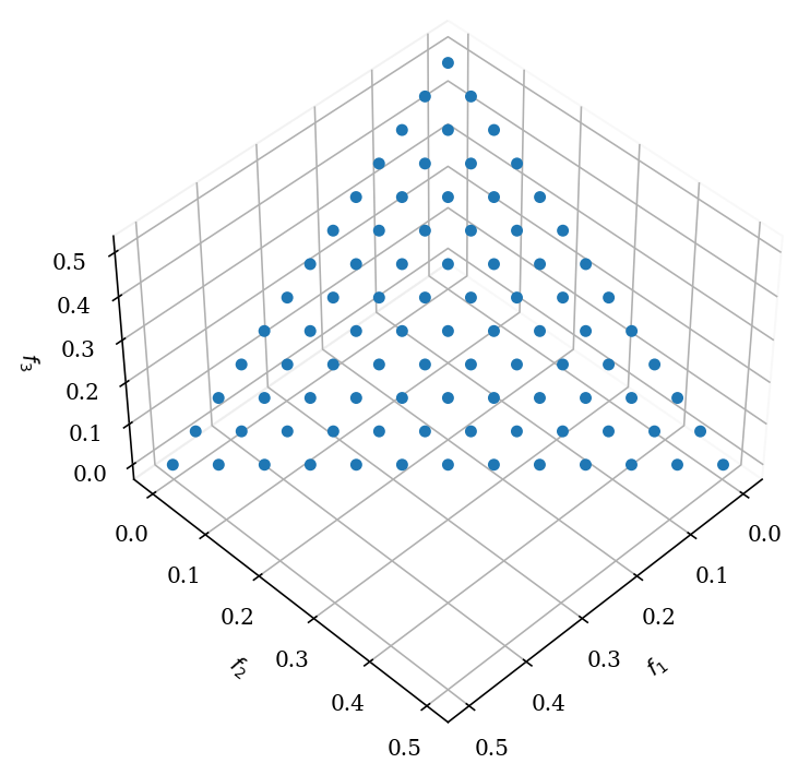
DTLZ1
The only difficulty provided by this problem is the convergence to the Pareto-optimal hyper-plane.The search space contains \((11^k-1)\) local Pareto-optimal fronts, where an MOEA can get attracted before reaching the global Pareto-optimal front.
Definition
\begin{equation} \newcommand{\boldx}{\mathbf{x}} \begin{array} \mbox{Minimize} & f_1(\boldx) = \frac{1}{2}x_1x_2\cdots x_{M-1}(1+g(\boldx_M)), \\ \mbox{Minimize} & f_2(\boldx) = \frac{1}{2}x_1x_2\cdots (1-x_{M-1})(1+g(\boldx_M)), \\ \vdots & \vdots \\ \mbox{Minimize} & f_{M-1}(\boldx) = \frac{1}{2}x_1 (1-x_2)(1+g(\boldx_M)), \\ \mbox{Minimize} & f_M(\boldx) = \frac{1}{2}(1-x_1) (1+g(\boldx_M)), \\[2mm] \mbox{subject to} & 0 \leq x_i \leq 1, \quad \mbox{for $i=1,2,\ldots,n$}. \end{array} \end{equation}
The last \(k=(n-M+1)\) variables are represented as \(\boldx_M\). The functional \(g(\boldx_M)\) requires \(|\boldx_M|=k\) variables and must take any function with \(g\geq 0\).
We suggest the following: \begin{equation} g(\boldx_M) = 100\left[|\boldx_M| + \sum_{x_i\in \boldx_M} (x_i-0.5)^2 - \cos(20 \pi (x_i-0.5)) \right] \end{equation}
Optimum
The Pareto-optimal solution corresponds to \(x_i=0.5\) (for all \(x_i\in \boldx_M\)) and the objective function values lie on the linear hyper-plane: \(\sum_{m=1}^M f_m^{\ast} = 0.5\).
Plot
[1]:
from pymoo.factory import get_problem, get_reference_directions, get_visualization
from pymoo.util.plotting import plot

ref_dirs = get_reference_directions("das-dennis", 3, n_partitions=12)

pf = get_problem("dtlz1").pareto_front(ref_dirs)
get_visualization("scatter", angle=(45,45)).add(pf).show()
[1]:
<pymoo.visualization.scatter.Scatter at 0x7f440ed5c520>
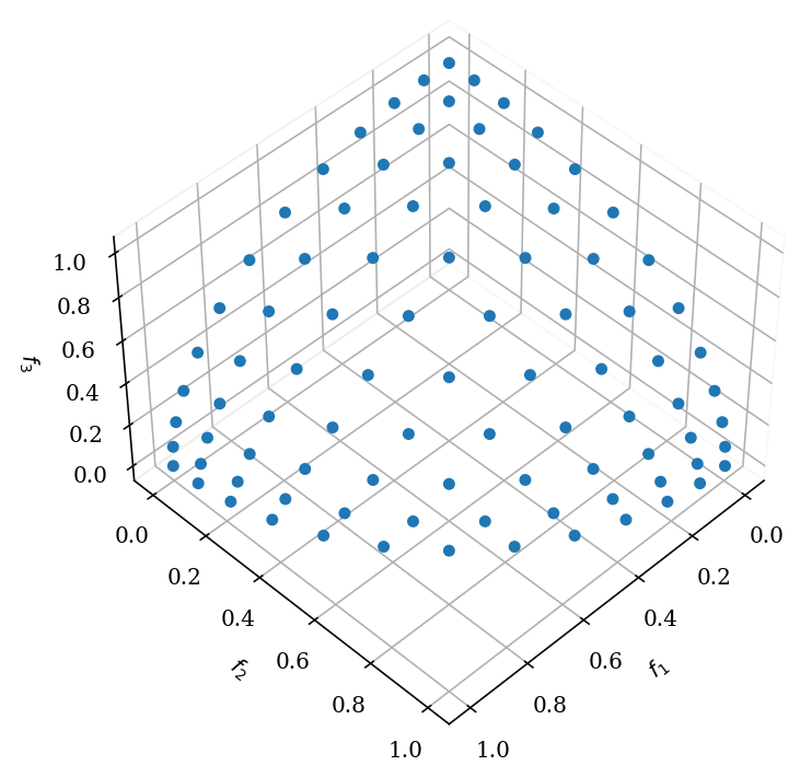
DTLZ2
This function can also be used to investigate an MOEA’s ability to scale up its performance in large number of objectives. Like in DTLZ1, for \(M>3\), the Pareto-optimal solutions must lie inside the first octant of the unit sphere in a three-objective plot with \(f_M\) as one of the axes. Since all Pareto-optimal solutions require to satisfy \(\sum_{m=1}^M f_m^2 = 1\), the difference between the left term with the obtained solutions and one can be used as a metric for convergence as well. Besides the suggestions given in DTLZ1, the problem can be made more difficult by replacing each variable \(x_i\) (for \(i=1\) to \((M-1)\)) with the mean value of \(p\) variables: \(x_i = \frac{1}{p}\sum_{k=(i-1)p+1}^{ip} x_k\).
Definition
\begin{equation} \begin{array} \mbox{Min.} & f_1(\boldx) = (1+g(\boldx_M)) \cos (x_1\pi/2) \cdots \cos (x_{M-2}\pi/2) \cos (x_{M-1}\pi/2), \\ \mbox{Min.} & f_2(\boldx) = (1+g(\boldx_M)) \cos (x_1\pi/2) \cdots \cos (x_{M-2}\pi/2) \sin (x_{M-1}\pi/2), \\ \mbox{Min.} & f_3(\boldx) = (1+g(\boldx_M)) \cos (x_1\pi/2) \cdots \sin (x_{M-2}\pi/2), \\ \vdots & \vdots \\ %\mbox{Min.} & f_{M-1}(\boldx) = (1+g(\boldx_M)) \cos (x_1\pi/2) \sin (x_2\pi/2), \\ \mbox{Min.} & f_{M}(\boldx) = (1+g(\boldx_M)) \sin (x_1\pi/2), \\[2mm] \mbox{with} & g(\boldx_M) = \sum_{x_i \in \boldx_M} (x_i-0.5)^2, \\[2mm] & 0 \leq x_i \leq 1, \quad \mbox{for $i=1,2,\ldots,n$}. \end{array} \end{equation}
Once again, the \(\boldx\) vector is constructed with \(k=n-M+1\) variables.
Optimum
The Pareto-optimal solutions corresponds to \(x_i=0.5\) for all \(x_i\in \boldx_M\).
Plot
[2]:
pf = get_problem("dtlz2").pareto_front(ref_dirs)
get_visualization("scatter", angle=(45,45)).add(pf).show()
[2]:
<pymoo.visualization.scatter.Scatter at 0x7f43fe994880>
DTLZ3
In order to investigate an MOEA’s ability to converge to the global Pareto-optimal front, we suggest using the above problem with the \(g\) function equal to Rastrigin. The \(g\) function introduces \((3^k-1)\) local Pareto-optimal fronts and one global Pareto-optimal front. All local Pareto-optimal fronts are parallel to the global Pareto-optimal front and an MOEA can get stuck at any of these local Pareto-optimal fronts, before converging to the global Pareto-optimal front (at \(g^{\ast}=0\)).
Definition
\begin{equation} \begin{array} \mbox{Min.} & f_1(\boldx) = (1+g(\boldx_M)) \cos (x_1\pi/2) \cdots \cos (x_{M-2}\pi/2) \cos (x_{M-1}\pi/2), \\ \mbox{Min.} & f_2(\boldx) = (1+g(\boldx_M)) \cos (x_1\pi/2) \cdots \cos (x_{M-2}\pi/2) \sin (x_{M-1}\pi/2), \\ \mbox{Min.} & f_3(\boldx) = (1+g(\boldx_M)) \cos (x_1\pi/2) \cdots \sin (x_{M-2}\pi/2), \\ \vdots & \vdots \\ %\mbox{Minimize} & f_{M-1}(\boldx) = (1+g(\boldx_M)) \cos (x_1\pi/2) \sin (x_2\pi/2), \\ \mbox{Min.} & f_{M}(\boldx) = (1+g(\boldx_M)) \sin (x_1\pi/2), \\ \mbox{with} & g(\boldx_M) = 100\left[|\boldx_M| + \sum_{x_i\in \boldx_M} (x_i-0.5)^2 - \cos(20 \pi (x_i-0.5))\right], \\ & 0 \leq x_i \leq 1, \quad \mbox{for $i=1,2,\ldots,n$}. \end{array} \end{equation}
Optimum
The global Pareto-optimal front corresponds to \(x_i = 0.5\) for \(x_i\in \boldx_M\).
Plot
[3]:
pf = get_problem("dtlz3").pareto_front(ref_dirs)
get_visualization("scatter", angle=(45,45)).add(pf).show()
[3]:
<pymoo.visualization.scatter.Scatter at 0x7f43fe8f4e50>

DTLZ4
In order to investigate an MOEA’s ability to maintain a good distribution of solutions, we modify problem DTLZ2 with a different parametric variable mapping:
Definition
\begin{equation} \begin{array} \mbox{Min.} & f_1(\boldx) = (1+g(\boldx_M)) \cos (x^{\alpha}_1\pi/2) \cdots \cos (x^{\alpha}_{M-2}\pi/2) \cos (x^{\alpha}_{M-1}\pi/2), \\ \mbox{Min.} & f_2(\boldx) = (1+g(\boldx_M)) \cos (x^{\alpha}_1\pi/2) \cdots \cos (x^{\alpha}_{M-2}\pi/2) \sin (x^{\alpha}_{M-1}\pi/2), \\ \mbox{Min.} & f_3(\boldx) = (1+g(\boldx_M)) \cos (x^{\alpha}_1\pi/2) \cdots \sin (x^{\alpha}_{M-2}\pi/2), \\ \vdots & \vdots \\ %\mbox{Minimize} & f_{M-1}(\boldx) = (1+g(\boldx_M)) \cos (x^{\alpha}_1\pi/2) \sin (x^{\alpha}_2\pi/2), \\ \mbox{Min.} & f_{M}(\boldx) = (1+g(\boldx_M)) \sin (x^{\alpha}_1\pi/2), \\ \mbox{with} & g(\boldx_M) = \sum_{x_i \in \boldx_M} (x_i-0.5)^2, \\[2mm] & 0 \leq x_i \leq 1, \quad \mbox{for $i=1,2,\ldots,n$}. \end{array} \end{equation}
The parameter \(\alpha=100\) is suggested here. This modification allows a dense set of solutions to exist near the \(f_M\)-\(f_1\) plane.
Optimum
The global Pareto-optimal front corresponds to \(x_i = 0.5\) for \(x_i\in \boldx_M\).
Plot
[4]:
pf = get_problem("dtlz4").pareto_front(ref_dirs)
get_visualization("scatter", angle=(45,45)).add(pf).show()
[4]:
<pymoo.visualization.scatter.Scatter at 0x7f43fe859580>

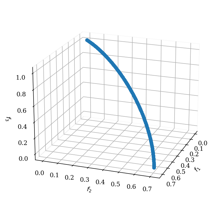
DTLZ5
This problem will test an MOEA’s ability to converge to a curve and will also allow an easier way to visually demonstrate (just by plotting \(f_M\) with any other objective function) the performance of an MOEA. Since there is a natural bias for solutions close to this Pareto-optimal curve, this problem may be easy for an algorithm to solve.
Definition
\begin{equation} \begin{array} \mbox{Min.} & f_1(\boldx) = (1+g(\boldx_M)) \cos (\theta_1\pi/2) \cdots \cos (\theta_{M-2}\pi/2) \cos (\theta_{M-1}\pi/2), \\ \mbox{Min.} & f_2(\boldx) = (1+g(\boldx_M)) \cos (\theta_1\pi/2) \cdots \cos (\theta_{M-2}\pi/2) \sin (\theta_{M-1}\pi/2), \\ \mbox{Min.} & f_3(\boldx) = (1+g(\boldx_M)) \cos (\theta_1\pi/2) \cdots \sin (\theta_{M-2}\pi/2), \\ \vdots & \vdots \\ %\mbox{Min.} & f_{M-1}(\boldx) = (1+g(\boldx_M)) \cos (\theta_1\pi/2) \sin (\theta_2\pi/2), \\ \mbox{Min.} & f_{M}(\boldx) = (1+g(\boldx_M)) \sin (\theta_1\pi/2), \\ \mbox{with} & \theta_i = \frac{\pi}{4(1+g(\boldx_M))}\left(1+2g(\boldx_M) x_i\right), \quad \mbox{for $i=2,3,\ldots,(M-1)$}, \\ & g(\boldx_M) = \sum_{x_i \in \boldx_M} (x_i-0.5)^2, \\ & 0 \leq x_i \leq 1, \quad \mbox{for $i=1,2,\ldots,n$}. \end{array} \end{equation}
Optimum
The Pareto-optimal front corresponds to \(x_i=0.5\) for all \(x_i\in \boldx_M\) and function values satisfy \(\sum_{m=1}^M f_m^2 = 1\).
Plot
[5]:
pf = get_problem("dtlz5").pareto_front()
get_visualization("scatter", angle=(20,20)).add(pf).show()
[5]:
<pymoo.visualization.scatter.Scatter at 0x7f43fe720070>

DTLZ6
The above test problem can be made harder by making a similar modification to the \(g\) function in DTLZ5, as done in DTLZ3.
Definition
However, in DTLZ6, we use a different \(g\) function:
\begin{equation} g(\boldx_M) = \sum_{x_i\in \boldx_M} x_i^{0.1}. \end{equation}
The size of \(\boldx_M\) vector is chosen as \(10\) and the total number of variables is identical as in DTLZ5. The above change in the problem makes NSGA-II and SPEA2 difficult to converge to the true Pareto-optimal front as in DTLZ5.
Optimum
Here, the Pareto-optimal front corresponds to \(x_i=0\) for all \(x_i\in \boldx_M\).
Plot
[6]:
pf = get_problem("dtlz6").pareto_front()
get_visualization("scatter", angle=(20,20)).add(pf).show()
[6]:
<pymoo.visualization.scatter.Scatter at 0x7f43fc2aa760>
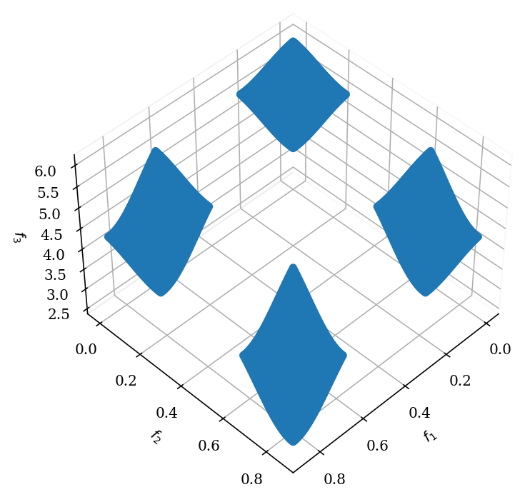
DTLZ7
This test problem has \(2^{M-1}\) disconnected Pareto-optimal regions in the search space. The functional \(g\) requires \(k=|\boldx_M|=n-M+1\) decision variables. This problem will test an algorithm’s ability to maintain subpopulation in different Pareto-optimal regions.
Definition
\begin{equation} \begin{array} \mbox{Minimize} & f_1(\boldx_1)=x_1, \\ \mbox{Minimize} & f_2(\boldx_2)=x_2, \\ \vdots & \vdots \\ \mbox{Minimize} & f_{M-1}(\boldx_{M-1})=x_{M-1}, \\ \mbox{Minimize} & f_M(\boldx) = (1+g(\boldx_M))h(f_1,f_2,\ldots,f_{M-1},g), \\ \mbox{where} & g(\boldx_M) = 1 + \frac{9}{|\boldx_M|}\sum_{x_i\in \boldx_M} x_i, \\ & h(f_1,f_2,\ldots,f_{M-1},g) = M-\sum_{i=1}^{M-1} \left[ \frac{f_i}{1+g}\left(1 + \sin (3\pi f_i)\right)\right], \\ \mbox{subject to} & 0 \leq x_i \leq 1, \quad \mbox{for $i=1,2,\ldots,n$}. \end{array} \end{equation}
Optimum
The Pareto-optimal solutions corresponds to \(\boldx_M=\vec{0}\).
Plot
[7]:
pf = get_problem("dtlz7").pareto_front()
get_visualization("scatter", angle=(45,45)).add(pf).show()
[7]:
<pymoo.visualization.scatter.Scatter at 0x7f43fe5c3790>