OSY
Osyczka and Kundu used the following six-variable test problem:
Definition
\begin{equation} \newcommand{\boldx}{\mathbf{x}} \begin{array} \mbox{Minimize} & f_1(\boldx) = -\left[25(x_1-2)^2+(x_2-2)^2 + (x_3-1)^2+(x_4-4)^2 + (x_5-1)^2\right], \\ \mbox{Minimize} & f_2(\boldx) = x_1^2 + x_2^2 + x_3^2 + x_4^2 + x_5^2 + x_6^2, \end{array} \end{equation}
\begin{equation} \begin{array} \mbox{\text{subject to}} & C_1(\boldx) \equiv x_1 + x_2 - 2 \geq 0, \\ & C_2(\boldx) \equiv 6 - x_1 - x_2 \geq 0, \\ & C_3(\boldx) \equiv 2 - x_2 + x_1 \geq 0, \\ & C_4(\boldx) \equiv 2 - x_1 + 3x_2 \geq 0, \\ & C_5(\boldx) \equiv 4 - (x_3-3)^2 - x_4 \geq 0, \\ & C_6(\boldx) \equiv (x_5-3)^2 + x_6 - 4 \geq 0, \\[2mm] & 0 \leq x_1,x_2,x_6 \leq 10,\quad 1 \leq x_3,x_5 \leq 5,\quad 0\leq x_4 \leq 6. \end{array} \end{equation}
Optimum
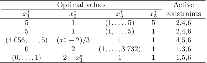
The Pareto-optimal region is a concatenation of five regions. Every region lies on some of the constraints. However, for the entire Pareto-optimal region, \(x_4^{\ast} = x_6^{\ast} = 0\). In table below shows the other variable values in each of the five regions and the constraints that are active in each region.
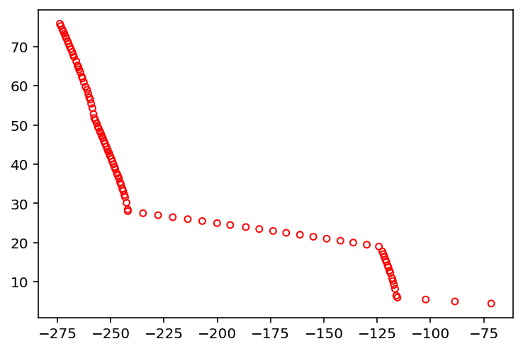
Plot
[1]:
from pymoo.factory import get_problem
from pymoo.util.plotting import plot

problem = get_problem("osy")
plot(problem.pareto_front(), no_fill=True)