TNK
Tanaka suggested the following two-variable problem:
Definition
\begin{equation} \newcommand{\boldx}{\mathbf{x}} \begin{array} \mbox{Minimize} & f_1(\boldx) = x_1, \\ \mbox{Minimize} & f_2(\boldx) = x_2, \\ \mbox{subject to} & C_1(\boldx) \equiv x_1^2 + x_2^2 - 1 - 0.1\cos \left(16\arctan \frac{x_1}{x_2}\right) \geq 0, \\ & C_2(\boldx) \equiv (x_1-0.5)^2 + (x_2-0.5)^2 \leq 0.5,\\ & 0 \leq x_1 \leq \pi, \\ & 0 \leq x_2 \leq \pi. \end{array} \end{equation}
Optimum
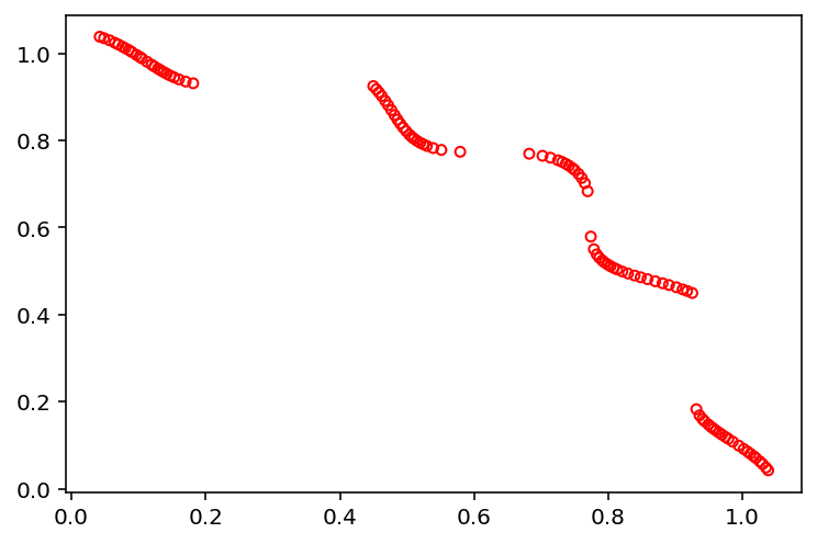
Since \(f_1=x_1\) and \(f_2=x_2\), the feasible objective space is also the same as the feasible decision variable space. The unconstrained decision variable space consists of all solutions in the square \(0\leq (x_1,x_2)\leq \pi\). Thus, the only unconstrained Pareto-optimal solution is \(x_1^{\ast}=x_2^{\ast}=0\). However, the inclusion of the first constraint makes this solution infeasible. The constrained Pareto-optimal solutions lie on the boundary of the first constraint. Since the constraint function is periodic and the second constraint function must also be satisfied, not all solutions on the boundary of the first constraint are Pareto-optimal. The Pareto-optimal set is disconnected. Since the Pareto-optimal solutions lie on a nonlinear constraint surface, an optimization algorithm may have difficulty in finding a good spread of solutions across all of the discontinuous Pareto-optimal sets.
Plot
[1]:
from pymoo.factory import get_problem
from pymoo.util.plotting import plot

problem = get_problem("tnk")
plot(problem.pareto_front(), no_fill=True)