DE: Differential Evolution¶

The classical single-objective differential evolution algorithm [14] where different crossover variations and methods can be defined. It is known for its good results for global optimization.

The differential evolution crossover is simply defined by:

\[v = x_{\pi_1} + F \cdot (x_{\pi_2} - x_{\pi_3})\]

where \(\pi\) is a random permutation with with 3 entries. The difference is taken between individual 2 and 3 and added to the first one. This is shown below:

de_crossover

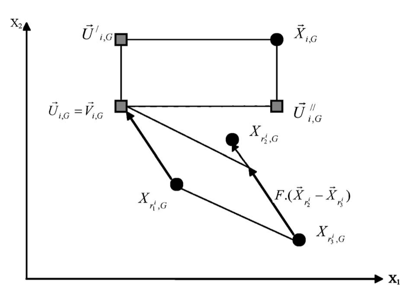
Then, a second crossover between an individual and the so-called donor vector \(v\) is performed. The second crossover can be simply binomial/uniform or exponential.

A great tutorial and more detailed information can be found here. The following guideline is copied from the description there (variable names are modified):

If you are going to optimize your own objective function with DE, you may try the following classical settings for the input file first: Choose method e.g. DE/rand/1/bin, set the population size to 10 times the number of parameters, select weighting factor F=0.8, and crossover constant CR=0.9. Recently, it has been found that selecting F from the interval (0.5, 1.0) randomly for each generation or each difference vector, a technique called dither, improves convergence behavior significantly, especially for noisy objective functions.

It has also been found that setting CR to a low value, e.g., CR=0.2 helps to optimize separable functions since it fosters the search along the coordinate axes. On the contrary, this choice is not effective if parameter dependence is encountered, which frequently occurs in real-world optimization problems rather than artificial test functions. So for parameter dependence, the choice of CR=0.9 is more appropriate. Another interesting empirical finding is that raising NP above, say, 40 does not substantially improve the convergence, independent of the number of parameters. It is worthwhile to experiment with these suggestions. Ensure that you initialize your parameter vectors by exploiting their full numerical range, i.e., if a parameter is allowed to exhibit values in the range (-100, 100), it is a good idea to pick the initial values from this range instead of unnecessarily restricting diversity.

Keep in mind that different problems often require different settings for NP, F, and CR (have a look into the different papers to get a feeling for the settings). If you still get misconvergence, you might want to try a different method. We mostly use ‘DE/rand/1/…’ or ‘DE/best/1/…’. The crossover method is not so crucial, although Ken Price claims that binomial is never worse than exponential. In the case of misconvergence, also check your choice of objective function. There might be a better one to describe your problem. Any knowledge that you have about the problem should be worked into the objective function. A good objective function can make all the difference.

And this is how DE can be used:

[1]:

from pymoo.algorithms.soo.nonconvex.de import DE
from pymoo.factory import get_problem
from pymoo.operators.sampling.lhs import LHS
from pymoo.optimize import minimize


problem = get_problem("ackley", n_var=10)


algorithm = DE(
    pop_size=100,
    sampling=LHS(),
    variant="DE/rand/1/bin",
    CR=0.3,
    dither="vector",
    jitter=False
)

res = minimize(problem,
               algorithm,
               seed=1,
               verbose=False)

print("Best solution found: \nX = %s\nF = %s" % (res.X, res.F))

Best solution found:
X = [ 2.07748676e-07  1.76803554e-07  4.19046439e-07 -7.33375135e-08
  1.11255737e-07  2.66003799e-07 -8.90155912e-08  2.02741800e-07
  2.66865482e-07  2.70503372e-07]
F = [9.22564873e-07]

API¶

class pymoo.algorithms.soo.nonconvex.de.DE(self, pop_size=100, n_offsprings=None, sampling=LHS(), variant='DE/best/1/bin', CR=0.5, F=None, dither='vector', jitter=False, mutation=NoMutation(), survival=None, display=SingleObjectiveDisplay(), **kwargs)

Parameters

pop_sizeint: The population sized used by the algorithm.
samplingSampling, Population, numpy.array: The sampling process defines the initial set of solutions which are the starting point of the optimization algorithm. Here, you have three different options by passing

(i) A Sampling implementation which is an implementation of a random sampling method.

(ii) A Population object containing the variables to be evaluated initially OR already evaluated solutions (F needs to be set in this case).

(iii) Pass a two dimensional numpy.array with (n_individuals, n_var) which contains the variable space values for each individual.
variant{DE/(rand|best)/1/(bin/exp)}: The different variants of DE to be used. DE/x/y/z where x how to select individuals to be pertubed, y the number of difference vector to be used and z the crossover type. One of the most common variant is DE/rand/1/bin.
Ffloat: The F to be used during the crossover.
CRfloat: The probability the individual exchanges variable values from the donor vector.
dither{‘no’, ‘scalar’, ‘vector’}: One strategy to introduce adaptive weights (F) during one run. The option allows the same dither to be used in one iteration (‘scalar’) or a different one for each individual (‘vector).
jitterbool: Another strategy for adaptive weights (F). Here, only a very small value is added or subtracted to the F used for the crossover for each individual.