Part II: Find a Solution Set using Multi-objective Optimization
The constrained bi-objective problem from Part I was defined by
\begin{align} \begin{split} \min \;\; & f_1(x) = 100 \, (x_1^2 + x_2^2) \\ \max \;\; & f_2(x) = -(x_1-1)^2 - x_2^2 \\[1mm] \text{s.t.} \;\; & g_1(x) = 2 \, (x_1 - 0.1) \, (x_1 - 0.9) \leq 0\\ & g_2(x) = 20 \, (x_1 - 0.4) \, (x_1 - 0.6) \geq 0\\[1mm] & -2 \leq x_1 \leq 2 \\ & -2 \leq x_2 \leq 2\\[1mm] & x \in \mathbb{R} \end{split} \end{align}
To implement the problem in pymoo some more work has to be done.
Problem Definition
Most optimization frameworks commit to either minimize or maximize all objectives and to have only \(\leq\) or \(\geq\) constraints. In pymoo, each objective function is supposed to be minimized, and each constraint needs to be provided in the form of \(\leq 0\).
Thus, we need to multiple an objective that is supposed to be maximized by \(-1\) and minimize it. This results in minimizing \(-f_2(x)\) instead of maximizing \(f_2(x)\).
Moreover, the inequality constraints need to be formulated as less than zero (\(\leq 0\)) constraint. For this reason, \(g_2(x)\) is multiplied by \(-1\) in order to flip inequality relation. Also, we recommend the normalization of constraints to make them operating on the same scale and giving them equal importance. For \(g_1(x)\), the coefficient results in \(2 \cdot (-0.1) \cdot (-0.9) = 0.18\) and for \(g_2(x)\) in \(20 \cdot (-0.4) \cdot (-0.6) = 4.8\), respectively. We achieve normalization of constraints by dividing \(g_1(x)\) and \(g_2(x)\) by its corresponding coefficient.
After these reformulations the problem to be implemented is given by:
\begin{align} \label{eq:getting_started_pymoo} \begin{split} \min \;\; & f_1(x) = 100 \, (x_1^2 + x_2^2) \\ \min \;\; & f_2(x) = (x_1-1)^2 + x_2^2 \\[1mm] \text{s.t.} \;\; & g_1(x) = 2 \, (x_1 - 0.1) \, (x_1 - 0.9) \, / \, 0.18 \leq 0\\ & g_2(x) = - 20 \, (x_1 - 0.4) \, (x_1 - 0.6) \, / \, 4.8 \leq 0\\[1mm] & -2 \leq x_1 \leq 2 \\ & -2 \leq x_2 \leq 2\\[1mm] & x \in \mathbb{R} \end{split} \end{align}
Implement the Problem
After having formulated the problem the right way, we can start implementing it. In this tutorial we the element-wise problem definition, which is one out of three different ways for implementing a problem. We define a new Python objective inheriting from ElementwiseProblem and set the correct attributes, such as the number of objectives (n_obj) and constraints (n_constr) and the lower (xl) and upper bounds (xu). The function being responsible for the evaluation is
_evaluate which shall be implemented next. The function’s interface is the parameters x and out. For this element-wise implementation x is a one-dimensional NumPy array of length n_var which represents a single solution to be evaluated. The output is supposed to be written to the dictionary out. The objective values should be written to out["F"] as a list of NumPy array with length of n_obj and the constraints to out["G"] with length of n_constr (if
the problem has constraints to be satisfied at all).
[1]:
import numpy as np
from pymoo.core.problem import ElementwiseProblem

class MyProblem(ElementwiseProblem):

    def __init__(self):
        super().__init__(n_var=2,
                         n_obj=2,
                         n_constr=2,
                         xl=np.array([-2,-2]),
                         xu=np.array([2,2]))

    def _evaluate(self, x, out, *args, **kwargs):
        f1 = 100 * (x[0]**2 + x[1]**2)
        f2 = (x[0]-1)**2 + x[1]**2

        g1 = 2*(x[0]-0.1) * (x[0]-0.9) / 0.18
        g2 = - 20*(x[0]-0.4) * (x[0]-0.6) / 4.8

        out["F"] = [f1, f2]
        out["G"] = [g1, g2]


problem = MyProblem()
Tip
A problem can be defined in a couple of different ways. Above, the implementation of an element-wise implementation is demonstrated, which means the _evaluate is called for each solution x at a time. Other ways of implementing a problem are vectorized, where x represents a whole set of solutions or a functional and probably more pythonic way by providing for each objective and constraint as a function. For more details, please have a look at the Problem tutorial.
If you use pymoo as a researcher trying to improve existing algorithms, you might want to have a look at the varierity of single- and many-objective optimization test problems already implemented.
Optimization Test Problems | Define a Custom Problem | Parallelization | Callback | Constraint Handling
Initialize an Algorithm
The reason why you became aware of this framework, is probably the existence of an algorithm you like to use. pymoo follows an object oriented approach and, thus, we have to define an algorithm object next. Depending on the optimization problem, different algorithms will perform better or worse on different kind of problems. It is recommendable to first understand the intuition behind an algorithm and then select one which seems to be most suitable for solving your optimization problem. A list of algorithms which are available in pymoo is available here.
In our case, the optimization problem is rather simple, but the aspect of having two objectives and two constraints should be considered. Thus, let us select the well-known multi-objective algorithm NSGA-II. For the majority of algorithms you could either choose the default hyper-parameters or create your own version of the algorithm by modifying them. For instance, for this relatively simple problem we choose a population size of 40 (pop_size=40) and with
only 10 (n_offsprings=10) in each generation. Such an implementation is a greedier variant and improves the convergence of simpler optimization problems without major difficulties regarding optimization, such as the existence of local Pareto-fronts. Moreover, we enable a duplicate check (eliminate_duplicates=True), making sure that the mating produces offsprings that are different from themselves and the existing population regarding their design space values.
[2]:
from pymoo.algorithms.moo.nsga2 import NSGA2
from pymoo.factory import get_sampling, get_crossover, get_mutation

algorithm = NSGA2(
    pop_size=40,
    n_offsprings=10,
    sampling=get_sampling("real_random"),
    crossover=get_crossover("real_sbx", prob=0.9, eta=15),
    mutation=get_mutation("real_pm", eta=20),
    eliminate_duplicates=True
)
The algorithm object contains an implementation of NSGA-II with the custom configuration discussed above. The object can now be used to start an optimization run.
Tip
The documentation is designed to make it easy to get started and to copy code for each of the algorithms. However, please be aware that each algorithm comes with all kinds of hyper-parameters to be considered. If an algorithm turns out not to show a good convergence behavior, we encourage you to try different algorithm configurations. For instance, for population-based approaches the population size and number of offsprings, as well as the parameters used for recombination operators are a good starting point.
Define a Termination Criterion
Furthermore, a termination criterion needs to be defined to start the optimization procedure. Most common ways of defining the termination is by limiting the overall number of function evaluations or simply the number of iterations of the algorithm. Moreover, some algorithms already have implemented their own, for instance Nelder-Mead when the simplex becomes degenerated or CMA-ES where a vendor library is used. Because of the simplicity of this problem we use a rather small number of 40 iteration of the algorithm.
[3]:
from pymoo.factory import get_termination

termination = get_termination("n_gen", 40)
Tip
A convergence analysis will show how much progress an algorithm has made at what time. Always keep in mind that having the most suitable algorithm but running it not long enough might prevent from finding the global optimum. However, continuing with optimization of an algorithm that got stuck or has already found the optimum will not improve the best found solution and unnecessarily increase the number of function evaluations.
You can find a list and explanations of termination criteria available in pymoo here. If no termination criteria is defined, then the progress in the design and objective space will kept track of in each iteration. When no significant progress has been made (this is the art of defining what that shall be), the algorithm terminates.
Optimize
Finally, we are solving the problem with the algorithm and termination we have defined. The functional interface uses the minimize method. By default, the minimize performs deep-copies of the algorithm and the termination object which guarantees they are not modified during the function call. This is important to ensure that repetitive function calls with the same random seed end up with the same results. When the algorithm has been terminated, the minimize function
returns a Result object.
[4]:
from pymoo.optimize import minimize

res = minimize(problem,
               algorithm,
               termination,
               seed=1,
               save_history=True,
               verbose=True)

X = res.X
F = res.F
=====================================================================================
n_gen |  n_eval |   cv (min)   |   cv (avg)   |  n_nds  |     eps      |  indicator
=====================================================================================
    1 |      40 |  0.00000E+00 |  2.36399E+01 |       1 |            - |            -
    2 |      50 |  0.00000E+00 |  1.15486E+01 |       1 |  0.00000E+00 |            f
    3 |      60 |  0.00000E+00 |  5.277918607 |       1 |  0.00000E+00 |            f
    4 |      70 |  0.00000E+00 |  2.406068542 |       2 |  1.000000000 |        ideal
    5 |      80 |  0.00000E+00 |  0.908316880 |       3 |  0.869706146 |        ideal
    6 |      90 |  0.00000E+00 |  0.264746300 |       3 |  0.00000E+00 |            f
    7 |     100 |  0.00000E+00 |  0.054063822 |       4 |  0.023775686 |        ideal
    8 |     110 |  0.00000E+00 |  0.003060876 |       5 |  0.127815454 |        ideal
    9 |     120 |  0.00000E+00 |  0.00000E+00 |       6 |  0.085921728 |        ideal
   10 |     130 |  0.00000E+00 |  0.00000E+00 |       7 |  0.015715204 |            f
   11 |     140 |  0.00000E+00 |  0.00000E+00 |       8 |  0.015076323 |            f
   12 |     150 |  0.00000E+00 |  0.00000E+00 |       7 |  0.026135665 |            f
   13 |     160 |  0.00000E+00 |  0.00000E+00 |      10 |  0.010026699 |            f
   14 |     170 |  0.00000E+00 |  0.00000E+00 |      11 |  0.011833783 |            f
   15 |     180 |  0.00000E+00 |  0.00000E+00 |      12 |  0.008294035 |            f
   16 |     190 |  0.00000E+00 |  0.00000E+00 |      14 |  0.006095993 |        ideal
   17 |     200 |  0.00000E+00 |  0.00000E+00 |      17 |  0.002510398 |        ideal
   18 |     210 |  0.00000E+00 |  0.00000E+00 |      20 |  0.003652660 |            f
   19 |     220 |  0.00000E+00 |  0.00000E+00 |      20 |  0.010131820 |        nadir
   20 |     230 |  0.00000E+00 |  0.00000E+00 |      21 |  0.005676014 |            f
   21 |     240 |  0.00000E+00 |  0.00000E+00 |      25 |  0.010464402 |            f
   22 |     250 |  0.00000E+00 |  0.00000E+00 |      25 |  0.000547515 |            f
   23 |     260 |  0.00000E+00 |  0.00000E+00 |      28 |  0.001050255 |            f
   24 |     270 |  0.00000E+00 |  0.00000E+00 |      33 |  0.003841298 |            f
   25 |     280 |  0.00000E+00 |  0.00000E+00 |      37 |  0.006664377 |        nadir
   26 |     290 |  0.00000E+00 |  0.00000E+00 |      40 |  0.000963164 |            f
   27 |     300 |  0.00000E+00 |  0.00000E+00 |      40 |  0.000678243 |            f
   28 |     310 |  0.00000E+00 |  0.00000E+00 |      40 |  0.000815766 |            f
   29 |     320 |  0.00000E+00 |  0.00000E+00 |      40 |  0.001500814 |            f
   30 |     330 |  0.00000E+00 |  0.00000E+00 |      40 |  0.014706442 |        nadir
   31 |     340 |  0.00000E+00 |  0.00000E+00 |      40 |  0.003554320 |        ideal
   32 |     350 |  0.00000E+00 |  0.00000E+00 |      40 |  0.000624123 |            f
   33 |     360 |  0.00000E+00 |  0.00000E+00 |      40 |  0.000203925 |            f
   34 |     370 |  0.00000E+00 |  0.00000E+00 |      40 |  0.001048509 |            f
   35 |     380 |  0.00000E+00 |  0.00000E+00 |      40 |  0.001121103 |            f
   36 |     390 |  0.00000E+00 |  0.00000E+00 |      40 |  0.000664461 |            f
   37 |     400 |  0.00000E+00 |  0.00000E+00 |      40 |  0.000761066 |            f
   38 |     410 |  0.00000E+00 |  0.00000E+00 |      40 |  0.000521906 |            f
   39 |     420 |  0.00000E+00 |  0.00000E+00 |      40 |  0.004652095 |        nadir
   40 |     430 |  0.00000E+00 |  0.00000E+00 |      40 |  0.000287847 |            f
If the verbose=True, some printouts during the algorithm’s execution are provided. This can very from algorithm to algorithm. Here, we execute NSGA2 on a problem where pymoo has no knowledge about the optimum. Each line represents one iteration. The first two columns are the current generation counter and the number of evaluations so far. For constrained problems, the next two columns show the minimum constraint violation (cv (min)) and the average constraint violation (cv (avg))
in the current population. This is followed by the number of non-dominated solutions (n_nds) and two more metrics which represents the movement in the objective space.
Tip
An algorithm can be executed by using the minimize interface as shown below. In order to have more control over the algorithm execution, pymoo also offers an object-oriented execution. For an example and a discussion of each’s pros and cons, please consult or algorithm tutorial.
Visualize
Analyzing the solutions being found by the algorithm is vital. Always a good start is visualizing the solutions to get a grasp of commonalities or if the Pareto-front is known to even check the convergence.
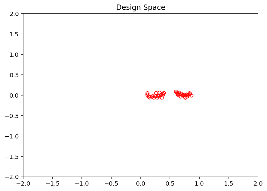
[5]:
import matplotlib.pyplot as plt
xl, xu = problem.bounds()
plt.figure(figsize=(7, 5))
plt.scatter(X[:, 0], X[:, 1], s=30, facecolors='none', edgecolors='r')
plt.xlim(xl[0], xu[0])
plt.ylim(xl[1], xu[1])
plt.title("Design Space")
plt.show()
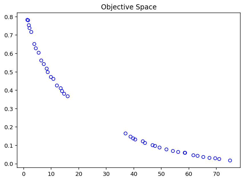
[6]:
plt.figure(figsize=(7, 5))
plt.scatter(F[:, 0], F[:, 1], s=30, facecolors='none', edgecolors='blue')
plt.title("Objective Space")
plt.show()