Part IV: Analysis of Convergence
Great! So far, we have executed an algorithm and already obtained a solution set. But let us not stop here without knowing how the algorithm has performed. This will also answer how we should define a termination criterion if we solve the problem again. The convergence analysis shall consider two cases, i) the Pareto-front is not known, or ii) the Pareto-front has been derived analytically, or a reasonable approximation exists.
Result
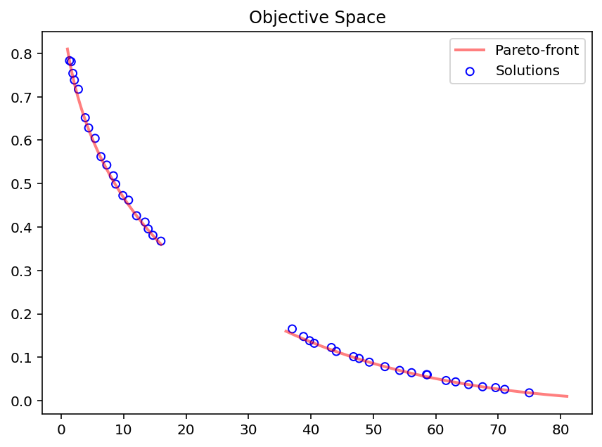
To further check how close the results match the analytically derived optimum, we have to convert the objective space values to the original definition where the second objective \(f_2\) was maximized. Plotting then the Pareto-front shows how close the algorithm was able to converge.
[2]:
from pymoo.util.misc import stack

class MyTestProblem(MyProblem):

    def _calc_pareto_front(self, flatten=True, *args, **kwargs):
        f2 = lambda f1: ((f1/100) ** 0.5 - 1)**2
        F1_a, F1_b = np.linspace(1, 16, 300), np.linspace(36, 81, 300)
        F2_a, F2_b = f2(F1_a), f2(F1_b)

        pf_a = np.column_stack([F1_a, F2_a])
        pf_b = np.column_stack([F1_b, F2_b])

        return stack(pf_a, pf_b, flatten=flatten)

    def _calc_pareto_set(self, *args, **kwargs):
        x1_a = np.linspace(0.1, 0.4, 50)
        x1_b = np.linspace(0.6, 0.9, 50)
        x2 = np.zeros(50)

        a, b = np.column_stack([x1_a, x2]), np.column_stack([x1_b, x2])
        return stack(a,b, flatten=flatten)

problem = MyTestProblem()
For IGD, the Pareto front needs to be known or to be approximated. In our framework, the Pareto front of test problems can be obtained by:
[3]:
pf_a, pf_b = problem.pareto_front(use_cache=False, flatten=False)
[4]:
pf = problem.pareto_front(use_cache=False, flatten=True)
[5]:
plt.figure(figsize=(7, 5))
plt.scatter(F[:, 0], F[:, 1], s=30, facecolors='none', edgecolors='b', label="Solutions")
plt.plot(pf_a[:, 0], pf_a[:, 1], alpha=0.5, linewidth=2.0, color="red", label="Pareto-front")
plt.plot(pf_b[:, 0], pf_b[:, 1], alpha=0.5, linewidth=2.0, color="red")
plt.title("Objective Space")
plt.legend()
plt.show()
Whether the optimum for your problem is known or not, we encourage all end-users of pymoo not to skip the analysis of the obtained solution set. Visualizations for high-dimensional objective spaces (in design and/or objective space) are also provided and shown here.
In Part II, we have run the algorithm without storing, keeping track of the optimization progress, and storing information. However, for analyzing the convergence, historical data need to be stored. One way of accomplishing that is enabling the save_history flag, which will store a deep copy of the algorithm object in each iteration and save it in the Result object. This approach is more memory-intensive (especially for many iterations) but has the advantage that any
algorithm-dependent variable can be analyzed posteriorly.
A not negligible step is the post-processing after having obtained the results. We strongly recommend not only analyzing the final result but also the algorithm’s behavior. This gives more insights into the convergence of the algorithm.
For such an analysis, intermediate steps of the algorithm need to be considered. This can either be achieved by:
A
Callbackclass storing the necessary information in each iteration of the algorithm.Enabling the
save_historyflag when calling the minimize method to store a deep copy of the algorithm’s objective each iteration.
We provide some more details about each variant in our convergence tutorial. As you might have already seen, we have set save_history=True when calling the minmize method in this getting started guide and, thus, will you the history for our analysis. Moreover, we need to decide what metric should be used to measure the performance of our algorithm. In this tutorial, we are going to use Hypervolume and IGD. Feel free to look at our performance
indicators to find more information about metrics to measure the performance of multi-objective algorithms.
[6]:
from pymoo.optimize import minimize

res = minimize(problem,
               algorithm,
               ("n_gen", 40),
               seed=1,
               save_history=True,
               verbose=False)

X, F = res.opt.get("X", "F")

hist = res.history
print(len(hist))
40
From the history it is relatively easy to extract the information we need for an analysis.
[7]:
n_evals = []             # corresponding number of function evaluations\
hist_F = []              # the objective space values in each generation
hist_cv = []             # constraint violation in each generation
hist_cv_avg = []         # average constraint violation in the whole population

for algo in hist:

    # store the number of function evaluations
    n_evals.append(algo.evaluator.n_eval)

    # retrieve the optimum from the algorithm
    opt = algo.opt

    # store the least contraint violation and the average in each population
    hist_cv.append(opt.get("CV").min())
    hist_cv_avg.append(algo.pop.get("CV").mean())

    # filter out only the feasible and append and objective space values
    feas = np.where(opt.get("feasible"))[0]
    hist_F.append(opt.get("F")[feas])
Constraint Satisfaction
First, let us quickly see when the first feasible solution has been found:
[8]:
k = np.where(np.array(hist_cv) <= 0.0)[0].min()
print(f"At least one feasible solution in Generation {k} after {n_evals[k]} evaluations.")
At least one feasible solution in Generation 0 after 40 evaluations.
Because this problem does not have much complexity, a feasible solution was found right away. Nevertheless, this can be entirely different for your optimization problem and is also worth being analyzed first.
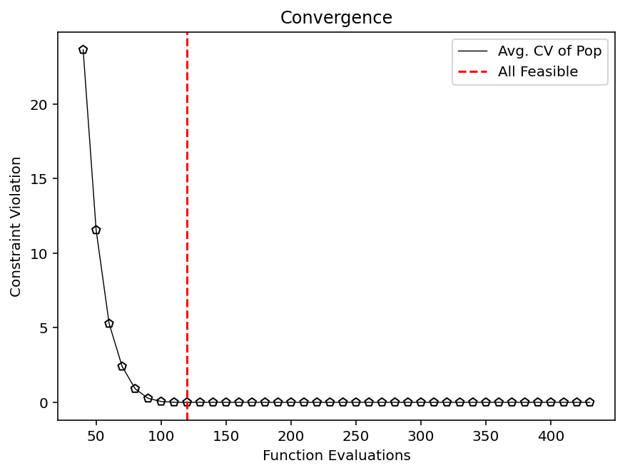
[9]:
# replace this line by `hist_cv` if you like to analyze the least feasible optimal solution and not the population
vals = hist_cv_avg

k = np.where(np.array(vals) <= 0.0)[0].min()
print(f"Whole population feasible in Generation {k} after {n_evals[k]} evaluations.")

plt.figure(figsize=(7, 5))
plt.plot(n_evals, vals,  color='black', lw=0.7, label="Avg. CV of Pop")
plt.scatter(n_evals, vals,  facecolor="none", edgecolor='black', marker="p")
plt.axvline(n_evals[k], color="red", label="All Feasible", linestyle="--")
plt.title("Convergence")
plt.xlabel("Function Evaluations")
plt.ylabel("Constraint Violation")
plt.legend()
plt.show()
Whole population feasible in Generation 8 after 120 evaluations.
Pareto-front is unknown
If the Pareto-front is not known, we can not know if the algorithm has converged to the true optimum or not. At least not without any further information. However, we can see when the algorithm has made most of its progress during optimization and thus if the number of iterations should be less or more. Additionally, the metrics serve to compare two algorithms with each other.
In multi-objective optimization normalization the very important. For that reason, you see below that the Hypervolume is based on a normalized set normalized by the bounds (idea) More details about it will be shown in Part IV.
Hypvervolume (HV)
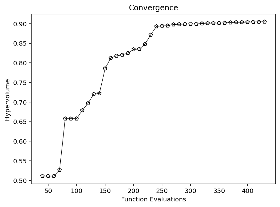
Hypervolume is a very well-known performance indicator for multi-objective problems. It is Pareto-compliant and is based on the volume between a predefined reference point and the solution provided. Therefore, hypervolume requires defining a reference point ref_point, which shall be larger than the maximum value of the Pareto front.
[10]:
approx_ideal = F.min(axis=0)
approx_nadir = F.max(axis=0)
[11]:
from pymoo.indicators.hv import Hypervolume

metric = Hypervolume(ref_point= np.array([1.1, 1.1]),
                     norm_ref_point=False,
                     zero_to_one=True,
                     ideal=approx_ideal,
                     nadir=approx_nadir)

hv = [metric.do(_F) for _F in hist_F]

plt.figure(figsize=(7, 5))
plt.plot(n_evals, hv,  color='black', lw=0.7, label="Avg. CV of Pop")
plt.scatter(n_evals, hv,  facecolor="none", edgecolor='black', marker="p")
plt.title("Convergence")
plt.xlabel("Function Evaluations")
plt.ylabel("Hypervolume")
plt.show()
Note: Hypervolume becomes computationally expensive with increasing dimensionality. The exact hypervolume can be calculated efficiently for 2 and 3 objectives. For higher dimensions, some researchers use a hypervolume approximation, which is not available yet in pymoo.
Running Metric
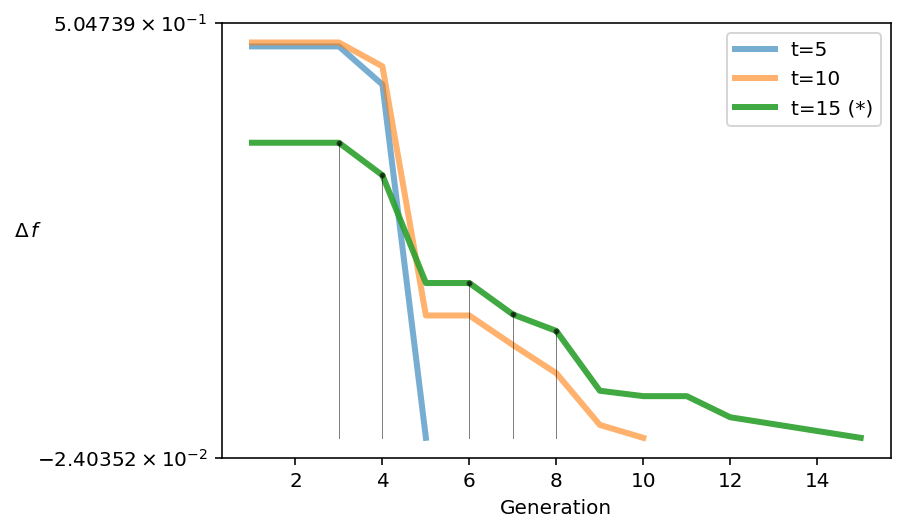
Another way of analyzing a run when the true Pareto front is not known is the recently proposed running metric. The running metric shows the difference in the objective space from one generation to another and uses the algorithm’s survival to visualize the improvement. This metric is also being used in pymoo to determine the termination of a multi-objective optimization algorithm if no default termination criteria have been defined.
For instance, this analysis reveals that the algorithm improved from the 4th to the 5th generation significantly.
[12]:
from pymoo.util.running_metric import RunningMetric

running = RunningMetric(delta_gen=5,
                        n_plots=3,
                        only_if_n_plots=True,
                        key_press=False,
                        do_show=True)

for algorithm in res.history[:15]:
    running.notify(algorithm)
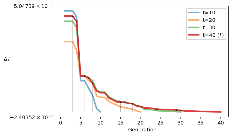
Plotting until the final population shows the algorithm seems to have more a less converged, and only a slight improvement has been made.
[13]:
from pymoo.util.running_metric import RunningMetric

running = RunningMetric(delta_gen=10,
                        n_plots=4,
                        only_if_n_plots=True,
                        key_press=False,
                        do_show=True)

for algorithm in res.history:
    running.notify(algorithm)
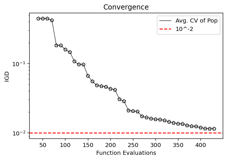
Pareto-front is known or approximated
IGD/GD/IGD+/GD+
The Pareto-front for a problem can either be provided manually or directly implemented in the Problem definition to analyze the run on the fly. Here, we show an example of using the history of the algorithm as an additional post-processing step.
For real-world problems, you have to use an approximation. An approximation can be obtained by running an algorithm a couple of times and extracting the non-dominated solutions out of all solution sets. If you have only a single run, an alternative is to use the obtained non-dominated set of solutions as an approximation. However, the result only indicates how much the algorithm’s progress in converging to the final set.
[14]:
from pymoo.indicators.igd import IGD

metric = IGD(pf, zero_to_one=True)

igd = [metric.do(_F) for _F in hist_F]

plt.plot(n_evals, igd,  color='black', lw=0.7, label="Avg. CV of Pop")
plt.scatter(n_evals, igd,  facecolor="none", edgecolor='black', marker="p")
plt.axhline(10**-2, color="red", label="10^-2", linestyle="--")
plt.title("Convergence")
plt.xlabel("Function Evaluations")
plt.ylabel("IGD")
plt.yscale("log")
plt.legend()
plt.show()
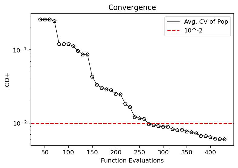
[15]:
from pymoo.indicators.igd_plus import IGDPlus

metric = IGDPlus(pf, zero_to_one=True)

igd = [metric.do(_F) for _F in hist_F]

plt.plot(n_evals, igd,  color='black', lw=0.7, label="Avg. CV of Pop")
plt.scatter(n_evals, igd,  facecolor="none", edgecolor='black', marker="p")
plt.axhline(10**-2, color="red", label="10^-2", linestyle="--")
plt.title("Convergence")
plt.xlabel("Function Evaluations")
plt.ylabel("IGD+")
plt.yscale("log")
plt.legend()
plt.show()