Source Code
In this guide, we have provided a couple of options for defining your problem and how to run the optimization. You might have already copied the code into your IDE. However, if not, the following code snippets cover the problem definition, algorithm initializing, solving the optimization problem, and visualization of the non-dominated set of solutions altogether.
[1]:
import numpy as np
from pymoo.algorithms.moo.nsga2 import NSGA2
from pymoo.core.problem import ElementwiseProblem
from pymoo.optimize import minimize
from pymoo.visualization.scatter import Scatter
class MyProblem(ElementwiseProblem):
def __init__(self):
super().__init__(n_var=2,
n_obj=2,
n_constr=2,
xl=np.array([-2, -2]),
xu=np.array([2, 2]))
def _evaluate(self, x, out, *args, **kwargs):
f1 = 100 * (x[0] ** 2 + x[1] ** 2)
f2 = (x[0] - 1) ** 2 + x[1] ** 2
g1 = 2 * (x[0] - 0.1) * (x[0] - 0.9) / 0.18
g2 = - 20 * (x[0] - 0.4) * (x[0] - 0.6) / 4.8
out["F"] = [f1, f2]
out["G"] = [g1, g2]
problem = MyProblem()
algorithm = NSGA2(pop_size=100)
res = minimize(problem,
algorithm,
("n_gen", 100),
verbose=False,
seed=1)
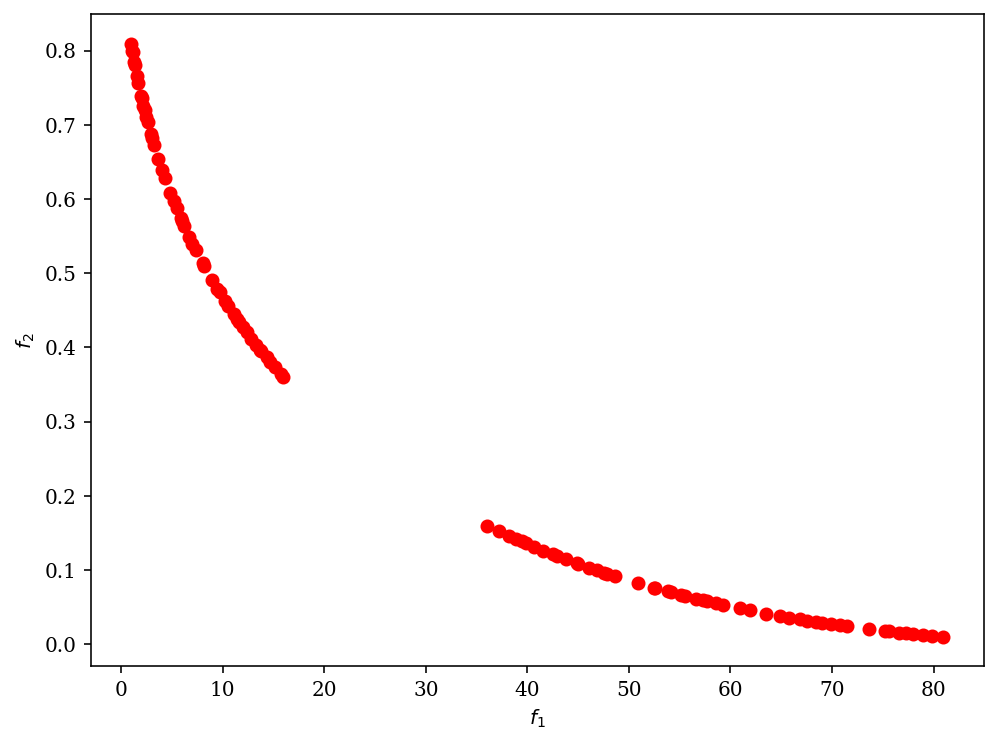
plot = Scatter()
plot.add(res.F, color="red")
plot.show()
[1]:
<pymoo.visualization.scatter.Scatter at 0x7f93ce8e0790>